Compare metrics across multiple time periods

Knowledge checkpoint

A grasp of these concepts will help you understand this documentation better:

• Logical Functions (case)
• where
• relative_period
• Natural Time Expressions
• Query Model
• AML Function
• String Interpolation

Introduction

Stakeholders often want a single summary view showing key business metrics side-by-side across several time windows, much like an executive scorecard or a KPI summary sheet in a spreadsheet.

For example, you might want to see GMV, NMV, AOV, total orders, delivered orders, cancelled orders, and cancellation rate for the current week, month-to-date (MTD), MTD last year, year-to-date (YTD), and YTD last year, all in one compact table.

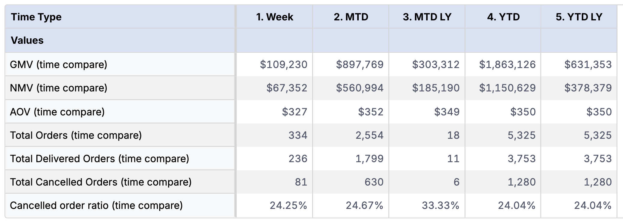
This pattern works for any type of metric, whether it's a monetary sum like GMV, a count like Total Orders, a ratio like AOV, or a percentage like Cancelled Order Ratio.

In this guide, we will walk you through how to build this kind of report in Holistics by combining a standalone query model, conditional metrics, and a Pivot Table.

High-level flow

Here is how the pieces fit together:

1. Create a Time Type query model. We build a standalone query model that generates one row per time period label (for e.g., Week, MTD, MTD LY, YTD, YTD LY). This model doesn't need any relationships to your fact tables.

2. Define conditional metrics using case(). For each metric (e.g., GMV), we write a case() expression that branches on the Time Type value. Each branch applies where() with a natural time expression like @(this week) or @(this year to today). For "last year" variants, we also apply relative_period() to shift the time window back by one year.

3. Visualize in a Pivot Table. We place the Time Type dimension in the Columns shelf and the metrics as Values (displayed as rows). This gives us the familiar spreadsheet-style layout.

Setup

For this guide, we use an ecommerce dataset with orders, order_items, products, users, and a date_dim. We also define several base metrics that we will later wrap with time-period logic.

ecommerce.dataset.aml

Dataset ecommerce {
  models: [
    orders, users, order_items, products, date_dim
  ]

  relationships: [
    relationship(orders.user_id > users.id, true),
    relationship(order_items.order_id > orders.id, true),
    relationship(order_items.product_id > products.id, true),
    relationship(orders.created_date > date_dim.date_key, true)
    // No relationship for time_type — it's intentionally standalone
  ]

  // --- Base metrics (these are what we'll wrap with time-period logic) ---

  metric gmv {  }

  metric nmv {  }

  metric total_orders {  }

  metric aov {  }

  metric total_delivered_orders {  }

  metric total_cancelled_orders {  }

  metric cancelled_order_ratio {  }

}

With these base metrics in place, we are ready to create the time-period variants.

Implementation

Step 1: Create the Time Type query model

The first step is to create a standalone query model that generates the time period labels. This model uses a simple SQL VALUES clause to produce one row per period. It doesn't need a relationship to your fact tables, as it serves as a virtual dimension table that provides column headers for the pivot.

We prefix each label with a number (e.g., 1. Week, 2. MTD) to control the sort order of columns in the final pivot table.

time_type.model.aml

Model time_type {
  type: 'query'
  label: 'Time Type'
  data_source_name: 'your_data_source'

  query: @sql
    SELECT time_type FROM (VALUES
      ('1. Week'),
      ('2. MTD'),
      ('3. MTD LY'),
      ('4. YTD'),
      ('5. YTD LY')
    ) AS t(time_type) ;;

  dimension time_type {
    label: 'Time Type'
    type: 'text'
    definition: @sql {{ #SOURCE.time_type }} ;;
  }
}

info

The VALUES syntax works on most modern databases (PostgreSQL, BigQuery, Snowflake, etc.). If your database doesn't support it, you can use UNION ALL instead:

SELECT '1. Week' AS time_type
UNION ALL SELECT '2. MTD'
UNION ALL SELECT '3. MTD LY'
UNION ALL SELECT '4. YTD'
UNION ALL SELECT '5. YTD LY'

Step 2: Add the Time Type model to the dataset

Once the model is created, add time_type to the models list of your dataset. You don't need to define any relationship for it

ecommerce.dataset.aml

Dataset ecommerce {
  ...

  models: [
    orders, users, order_items, products, date_dim,
    time_type  // standalone — no relationship needed
  ]

  relationships: [
    // your existing relationships stay the same
    relationship(orders.user_id > users.id, true),
    relationship(order_items.order_id > orders.id, true),
    ...
  ]
}

Step 3: Define conditional metrics

Now we define metrics that compute different values depending on which time period is active. The case() function branches on time_type.time_type, and each branch uses where() with a natural time expression to filter the date range. For "last year" variants, we pipe through relative_period() to shift the window back by one year.

Here is what each branch does:

Branch	Time Expression	Meaning
1. Week	@(this week)	Current calendar week
2. MTD	@(this month to today)	Start of current month through today
3. MTD LY	relative_period + @(this month to today)	Same month-to-date window, shifted 1 year back
4. YTD	@(this year to today)	Start of current year through today
5. YTD LY	relative_period + @(this year to today)	Same year-to-date window, shifted 1 year back

Here are two examples (GMV and Total Orders), showing how the pattern works:

ecommerce.dataset.aml

Dataset ecommerce {
  ...

  metric gmv_time_compare {
      label: 'GMV (time compare)'
      type: 'number'
      definition: @aql case(
          when: time_type.time_type == "1. Week"
          , then: gmv | where(date_dim.date_key match @(this week))
          , when: time_type.time_type == "2. MTD"
          , then: gmv | where(date_dim.date_key match @(this month to today))
          , when: time_type.time_type == "3. MTD LY"
          , then: gmv | relative_period(date_dim.date_key, interval(-1 year)) | where(date_dim.date_key match @(this month to today))
          , when: time_type.time_type == "4. YTD"
          , then: gmv | where(date_dim.date_key match @(this year to today))
          , when: time_type.time_type == "5. YTD LY"
          , then: gmv | relative_period(date_dim.date_key, interval(-1 year)) | where(date_dim.date_key match @(this year to today))
      ) ;;
      format: "[$]#,###0"
  }

  metric total_orders_time_compare {
      label: 'Total Orders (time compare)'
      type: 'number'
      definition: @aql case(
          when: time_type.time_type == "1. Week"
          , then: total_orders | where(date_dim.date_key match @(this week))
          , when: time_type.time_type == "2. MTD"
          , then: total_orders | where(date_dim.date_key match @(this month to today))
          , when: time_type.time_type == "3. MTD LY"
          , then: total_orders | relative_period(date_dim.date_key, interval(-1 year)) | where(date_dim.date_key match @(this month to today))
          , when: time_type.time_type == "4. YTD"
          , then: total_orders | where(date_dim.date_key match @(this year to today))
          , when: time_type.time_type == "5. YTD LY"
          , then: total_orders | relative_period(date_dim.date_key, interval(-1 year)) | where(date_dim.date_key match @(this year to today))
      ) ;;
      format: "#,###"
  }

  // ... same pattern for nmv, aov, total_delivered_orders, cancelled_order_ratio, etc.

}

Notice how the two metrics are nearly identical, only the base metric name (gmv vs total_orders), the label, and the format differ. The case() structure and the relative_period() / where() logic are exactly the same. For "last year" branches, we apply relative_period(date_dim.date_key, interval(-1 year)) first to shift the time window, then where() to filter the date range.

As you add more metrics, this copy-paste pattern quickly becomes hard to maintain.

Reduce repetition with AML Func

Instead of duplicating this block for every metric, we can use an AML Function with string interpolation to extract the pattern into a reusable function.

Define the function in a separate file (or at the top of your dataset file):

time_compare_func.aml

Func time_compare(metric_name: String, metric_label: String, format: String) {
  Metric {
    label: '${metric_label} (time compare)'
    type: 'number'
    definition: @aql case(
        when: time_type.time_type == "1. Week"
        , then: ${metric_name} | where(date_dim.date_key match @(this week))
        , when: time_type.time_type == "2. MTD"
        , then: ${metric_name} | where(date_dim.date_key match @(this month to today))
        , when: time_type.time_type == "3. MTD LY"
        , then: ${metric_name} | relative_period(date_dim.date_key, interval(-1 year)) | where(date_dim.date_key match @(this month to today))
        , when: time_type.time_type == "4. YTD"
        , then: ${metric_name} | where(date_dim.date_key match @(this year to today))
        , when: time_type.time_type == "5. YTD LY"
        , then: ${metric_name} | relative_period(date_dim.date_key, interval(-1 year)) | where(date_dim.date_key match @(this year to today))
      )  ;;
    format: format
  }
}

The function takes three parameters:

• metric_name: the name of the base metric to wrap (e.g., 'gmv', 'total_orders')
• metric_label: the display label (e.g., 'GMV', 'Total Orders')
• format: the number format string

Inside the function, ${metric_name} and ${metric_label} are injected into the metric definition via string interpolation.

Now each metric declaration becomes a single line:

ecommerce.dataset.aml

Dataset ecommerce {
  ...

  // time comparison metrics
  metric gmv_time_compare: time_compare('gmv', 'GMV', '[$]#,###0')
  metric nmv_time_compare: time_compare('nmv', 'NMV', '[$]#,###0')
  metric aov_time_compare: time_compare('aov', 'AOV', '[$]#,###0')
  metric total_orders_time_compare: time_compare('total_orders', 'Total Orders', '#,###')
  metric total_delivered_orders_time_compare: time_compare('total_delivered_orders', 'Total Delivered Orders', '#,###')
  metric total_cancelled_orders_time_compare: time_compare('total_cancelled_orders', 'Total Cancelled Orders', '#,###')
  metric cancelled_order_ratio_time_compare: time_compare('cancelled_order_ratio', 'Cancelled Order Ratio', '#,###0.00%')
}

Adding a new metric to the scorecard is now a one-liner, no more copy-pasting 15 lines of case() logic.

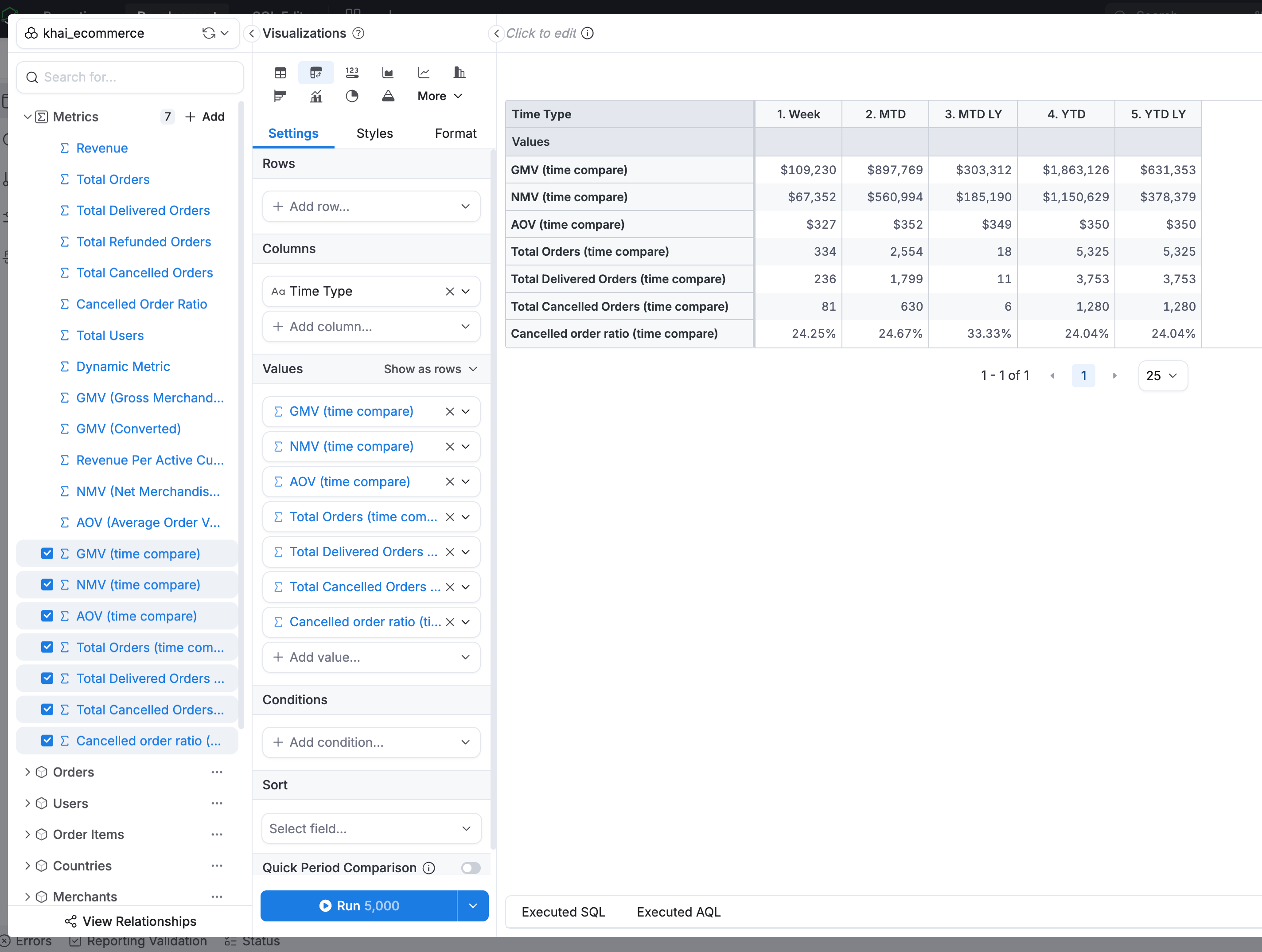
Step 4: Build the pivot table

With the model and metrics in place, create an exploration and set up the visualization:

1. Add time_type.time_type to the Columns shelf.
2. Add your time-compare metrics (e.g., gmv_time_compare, nmv_time_compare, aov_time_compare, total_orders_time_compare, cancelled_order_ratio_time_compare) as Values.
3. Set the chart type to Pivot Table.
4. In the Values section, switch to Show as rows so each metric becomes its own row.

Customization ideas

This pattern is flexible. Here are some ways you can adapt it:

• Different time periods. Add or replace case() branches for windows like QTD, QTD LY, Last Week, or Last Month. Just add corresponding rows in the time_type query model and matching when: branches in each metric.

• More metrics. Apply the same case() pattern to any base measure (revenue per active customer, refund rate, etc). Each new metric follows the identical structure.

• Custom sort order. The number prefixes (1., 2., etc.) control column ordering in the pivot. Adjust or remove them depending on how you want the columns arranged.