Moving Average

Moving averages smooth out fluctuations in a time series so the underlying trend is easier to see. This page builds a 3-month moving average of monthly revenue two ways: with trailing_period() and with window_avg(). It explains when to pick which.

Uses the shared e-commerce schema: orders, order_items, products.

Which function to use?

	trailing_period()	window_avg()
Operates on	Calendar time	Table rows
Handles gaps in data	Yes. uses the calendar, not the rows	No. Uses adjacent rows regardless of dates
Mixed time grains (e.g. metric defined on day, viz on month)	Yes	No. viz grain must match
Affected by visual filters	No. Computed before filters	Yes. Only sees visible rows

For example, with gaps in the data:

Month	Revenue	trailing_period (3M)	window_avg (3 rows)
Jan	100	100	100
Mar	100	50	100
Jun	100	50	100

trailing_period divides Mar's revenue by 3 because Feb and Apr are empty months. window_avg averages the three visible rows regardless of how far apart they are.

Default to trailing_period() for time-based moving averages. Reach for window_avg() when you genuinely want row-based logic (e.g. last-3-orders rather than last-3-months).

Setup

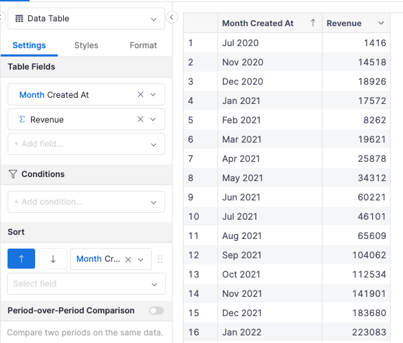
Start with a plain revenue metric on the e-commerce dataset:

Dataset e_commerce {
  metric revenue {
    label: 'Revenue'
    type: 'number'
    definition: @aql order_items | sum(order_items.quantity * products.price) ;;
  }
}

Option 1: trailing_period()

trailing_period() re-aggregates revenue over a moving calendar window. Two things to decide:

• The time dimension: the field that defines "which period a row belongs to." Use orders.created_at (no need to convert to month grain; the interval argument handles that).
• The window: interval(3 months) for a 3-month trailing window.

Because trailing_period() returns the sum over the window, divide by 3 to get the average:

metric moving_avg_revenue_3m_tp {
  label: '3M Moving Avg. Revenue (trailing_period)'
  type: 'number'
  definition: @aql trailing_period(revenue, orders.created_at, interval(3 months)) / 3 ;;
}

The first two rows look low because only 1 and 2 months of revenue exist within their windows. Filter them out in the visualization if that's confusing.

Option 2: window_avg()

window_avg() averages adjacent rows. You need to tell it:

• The frame: -2..0 means "from 2 rows back through the current row" (3 rows total).
• The order: orders.created_at | month() so rows are ordered by month before the window is applied.

metric moving_avg_revenue_3m_wa {
  label: '3M Moving Avg. Revenue (window_avg)'
  type: 'number'
  definition: @aql window_avg(revenue, -2..0, order: orders.created_at | month()) ;;
}

The first two rows average 1 and 2 rows respectively. To NULL them out instead, gate on window_count:

metric moving_avg_revenue_3m_wa {
  label: '3M Moving Avg. Revenue (window_avg)'
  type: 'number'
  definition: @aql case(
    when: window_count(revenue, -2..0, order: orders.created_at | month()) < 3,
    then: null,
    else: window_avg(revenue, -2..0, order: orders.created_at | month())
  ) ;;
}

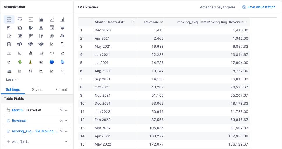
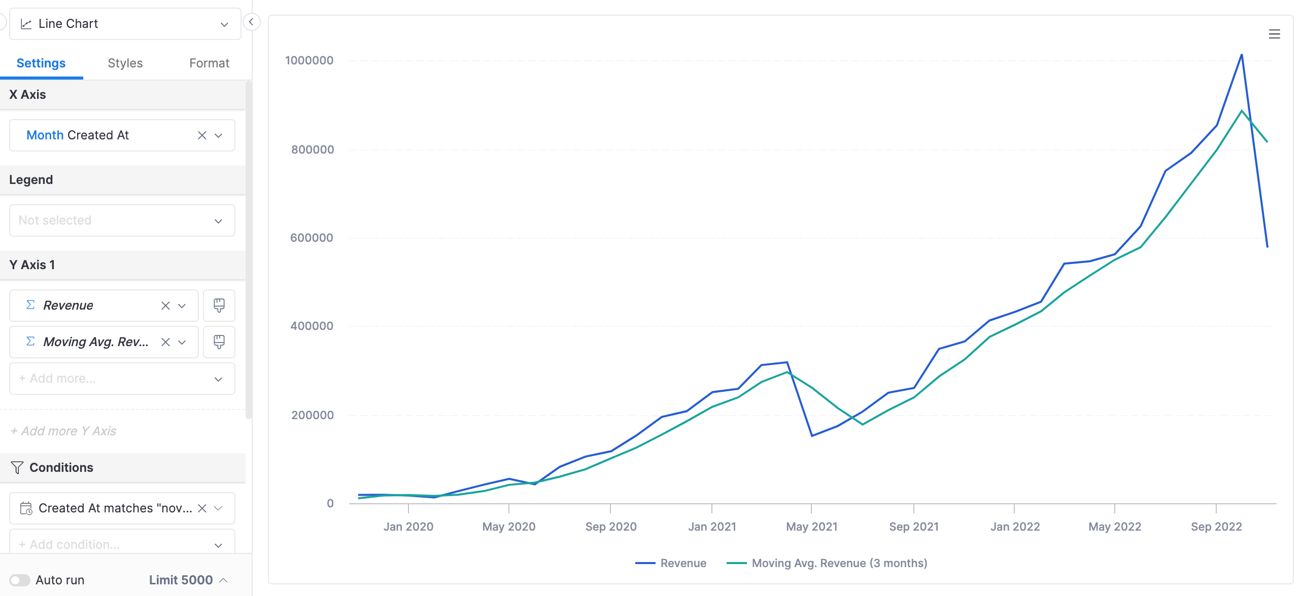
Visualize

Plot revenue and the moving average together. The smoothed line makes the trend much easier to read:

See also

• trailing_period: function reference
• window_avg: function reference
• Cumulative Metrics: running totals and accumulation
• Period Comparison: YoY, QoQ, and CAGR