Level of Detail Patterns

For the concept, vocabulary, and decision table, see Learn AQL → Level of Detail. This page walks through four real-world patterns end to end.

The simplest LoD case (percent of total with of_all()) has its own dedicated page: Percent of Total. The patterns below cover the trickier shapes.

Nested aggregation vs dimensionalize()

These two come up most often, and on the surface they can produce similar results. They behave differently under filters:

• Use dimensionalize() when you want the aggregation usable as a group-able dimension (bins, histograms, cohort buckets).
• Use nested aggregation for everything else. It's the more intuitive default.

A concrete difference: with a filter like orders.created_at matches 'last month', "Max of (AOV measure)" computes AOV from only last month's orders, while "Max of (AOV dimension via dimensionalize)" computes AOV across all-time orders for users who placed an order last month.

Use case 1: higher LoD. nested aggregation

Question: "What is the maximum AOV (average order value) of a customer in each country?"

Two-step calculation:

1. AOV per customer (high Calc LoD: needs users.id).
2. Max of those AOVs grouped by country.

The customer-level AOV measure:

Model users {
  measure aov {
    definition: @aql
      sum(order_items, order_items.quantity * products.price) * 1.0
      / count_distinct(orders.id)
    ;;
  }
}

The dataset-level metric that nests it:

Dataset ecommerce {
  metric max_user_aov {
    definition: @aql users | group(users.id) | select(user_aov: users.aov) | max() ;;
  }
}

When the report groups by country, AQL first computes AOV per user, then takes the max within each country group.

Use case 2: fixed LoD. dimensionalize()

Question: "Show countries colored by the highest customer AOV available there."

Here AOV behaves like a customer-level property, not a measure that recomputes per report. Define it as a dimension fixed to users.id:

Model users {
  dimension aov_dim {
    type: 'number'
    definition: @aql
      sum(order_items, order_items.quantity * products.price) * 1.0
      / count_distinct(orders.id)
      | dimensionalize(users.id)
    ;;
  }
}

And in the dataset:

Dataset ecommerce {
  metric max_user_aov {
    definition: @aql max(users.aov_dim) ;;
  }
}

Same shape as use case 1, but the AOV is locked to the user grain. See the comparison note above for when this matters.

Use case 3: customer segmentation flag. dimensionalize() for filtering

Question: "Identify VIP customers (lifetime revenue > $10k and 5+ orders), then break down orders by VIP vs. non-VIP."

This is dimensionalize() applied to a boolean expression. The aggregation collapses to a per-customer flag that other reports can filter and group by.

dimension is_vip_customer {
  model: users
  label: 'Is VIP Customer'
  type: 'truefalse'
  definition: @aql
    (sum_revenue > 10000 and count(orders.id) >= 5)
    | dimensionalize(users.id)
  ;;
}

Now any report can filter on users.is_vip_customer is true or group by it. The flag is fixed to the user grain regardless of what the surrounding report does. That's the point of dimensionalize().

Same shape as use case 2, but the output is a category, not a number.

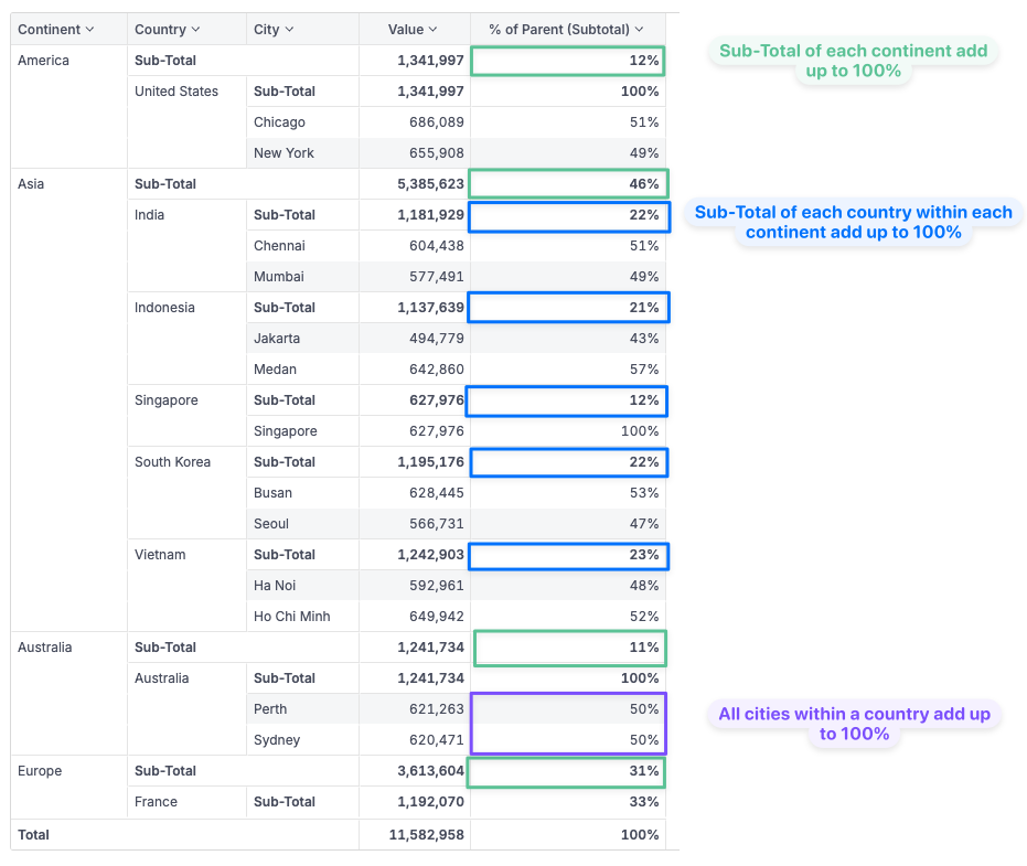
Use case 4: per-level percentages. is_at_level()

Question: In a pivot with Continent → Country → City, compute percent-of-parent at every level.

case(
  when: is_at_level(cities.name),
    then: sum(sales.amount) / (sum(sales.amount) | of_all(cities.name)),
  when: is_at_level(countries.name),
    then: sum(sales.amount) / (sum(sales.amount) | of_all(countries.name)),
  when: is_at_level(countries.continent),
    then: sum(sales.amount) / (sum(sales.amount) | of_all(countries.continent)),
  else: 1
)

is_at_level() detects which dimension is active and picks the right denominator. The else: 1 covers the Grand Total row.

See also

• of_all(): function reference
• dimensionalize(): function reference
• Nested aggregation guide
• Percent of total guide